In this post I’ll talk in detail about the forward path implementation of the famous AlexNet. This Convolutional Neural Network (CNN) by Krizhevsky and Hinton has won the ILSVR 2012 competition with a remarkable margin. If you are starting to work with CNNs or Deep Learning in general, this post will give you a head start. You can find a straight forward implementation of the CNN’s forward path on our Github site. Feel free to download it and classify arbitrary images.
When I was looking for more information on AlexNet and its implementation, I found a lot of information on UC Berkeley’s Caffe web page. They offer a definition of the network as well as pretrained weights. Additional useful information can be found in Stanford’s Deep Learning Tutorial as well as on Wikipedia.
The CNN by Alex Krizhevsky consists of 5 convolutional layers and 3 fully connected layers. Additionally each layer can be followed by a ReLU activation function, a maxpooling function for subsampling as well as by an LRN normalization. The exact definition of this CNN can be found here, with some explanation here. What follows is a description of all the different layer types.
Convolutional Layer
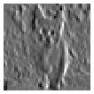
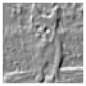
This layer convolves input feature maps with kernels, thus extracting different features. The first convolution layers will obtain the low-level features, like edges, lines and corners. The more layers the network has, the higher-level features it will get.
- Parameters:
Kernel size K: The kernels have dimension K x K.
Stride S: The kernels are applied at an interval of size S.
Padding pad: The input feature maps are padded at the edges with pad pixels (zero-initialized).
Group g: The input and output feature maps are split into g independent groups. - Example Features:
ReLU Nonlinearity (Rectified Linear Units)
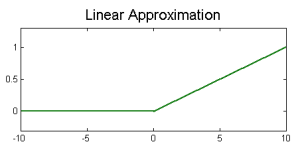
ReLU serves as activation function and speeds up training. Although other Nonlinearities such as sigmoid and tanh do exist, most successful CNNs use the fast ReLU.
- Formula:
Maxpooling
Since considering all extracted features would be computationally challenging, pooling layers are used to average these features over an image region. Additionally these layers help reduce over-fitting.
- Parameters:
Kernel size K: Specifies the pooling size.
Stride S: The pooling filter is applied in intervals of S.
Local Response Normalization (LRN)
LRN across channels normalizes inputs over adjacent feature maps. The normalization region includes pixels at nearby feature maps with the same x/y coordinates.
- Parameters:
Local Size n: The normalization region has dimension n x 1 x 1.
Alpha α, Beta β, Constant K: Scaling parameters. - Formula: Denoting
as the input at position (x,y) in feature map i, the output is computed as follows:
Fully Connected Layer
Fully connected layers convert input to output vectors.
- Formula:
Softmax Layer
The softmax function as the last layer computes the categorical probabilities. The sum of the output vector is 1.
- Formula:


